파이썬 데이터 사이언스 Cheat Sheet: NumPy 기초, 기본
파이썬 기반 데이터 분석 환경에서 NumPy1는 행렬 연산을 위한 핵심 라이브러리입니다. NumPy는 “Numerical Python“의 약자로 대규모 다차원 배열과 행렬 연산에 필요한 다양한 함수를 제공합니다. 특히 메모리 버퍼에 배열 데이터를 저장하고 처리하는 효율적인 인터페이스를 제공합니다. 파이썬 list 객체를 개선한 NumPy의 ndarray 객체를 사용하면 더 많은 데이터를 더 빠르게 처리할 수 있습니다.
NumPy는 다음과 같은 특징을 갖습니다.
- 강력한 N 차원 배열 객체
- 정교한 브로드케스팅(Broadcast) 기능
- C/C ++ 및 포트란 코드 통합 도구
- 유용한 선형 대수학, 푸리에 변환 및 난수 기능
- 범용적 데이터 처리에 사용 가능한 다차원 컨테이너
본 문서는 cs231n 강좌의 Python Numpy Tutorial 문서와 DataCamp의 Python For Data Science Cheat Sheet NumPy Basics 문서를 참조하여 작성하였습니다.
1. NumPy 배열
NumPy는 과학 연산을 위한 파이썬 핵심 라이브러리입니다. NumPy는 고성능 다차원 배열과 이런 배열을 처리하는 다양한 함수와 툴을 제공합니다.
파이썬에서 NumPy를 사용할 때, 다음과 같이 numpy 모듈을 “np”로 임포트하여 사용합니다.
import numpy as np
NumPy 라이브러리 버전은 다음과 같이 확인 할 수 있습니다.
import numpy as np
np.__version__
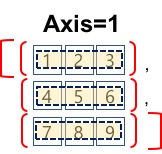
NumPy 배열은 <그림 1>과 같이 다차원 배열을 지원합니다. NumPy 배열의 구조는 “Shape“으로 표현됩니다. Shape은 배열의 구조를 파이썬 튜플 자료형을 이용하여 정의합니다. 예를 들어 28X28 컬러 사진은 높이가 28, 폭이 28, 각 픽셀은 3개 채널(RGB)로 구성된 데이터 구조를 갖습니다. 즉 컬러 사진 데이터는 Shaep이 (28, 28, 3)인 3차원 배열입니다. 다차원 배열은 입체적인 데이터 구조를 가지며, 데이터의 차원은 여러 갈래의 데이터 방향을 갖습니다. 다차원 배열의 데이터 방향을 axis로 표현할 수 있습니다. 행방향(높이), 열방향(폭), 채널 방향은 각각 axis=0, axis=1 그리고 axis=2로 지정됩니다. NumPy 집계(Aggregation) 함수는 배열 데이터의 집계 방향을 지정하는 axis 옵션을 제공합니다.
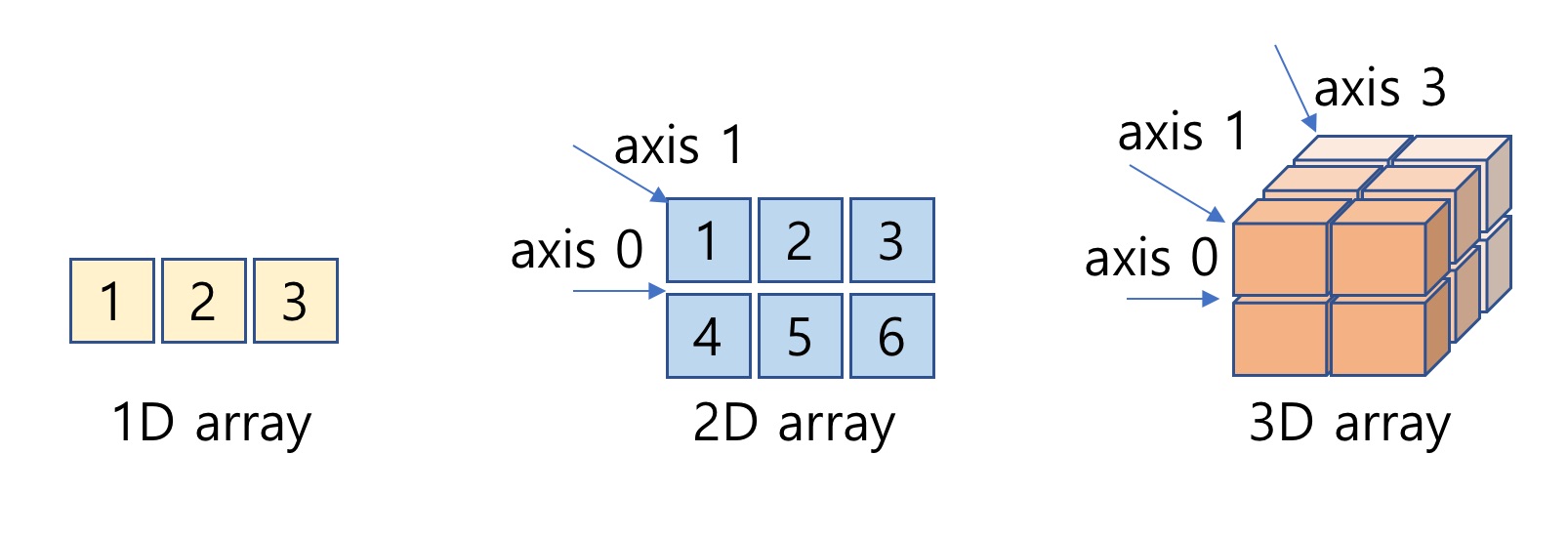
그림 1: NumPy 1차원, 2차원 및 3차원 배열과 Axis
NumPy 배열의 axis와 관련해서는 “Numpy에서 np.sum 함수의 axis 이해” 문서를 참조하시기 바랍니다.
본 문서에서는 NumPy 객체의 정보를 출력하는 용도로 다음 pprint 함수를 공통으로 사용합니다.
def pprint(arr):
    print("type:{}".format(type(arr)))
    print("shape: {}, dimension: {}, dtype:{}".format(arr.shape, arr.ndim, arr.dtype))
    print("Array's Data:\n", arr)
2. 배열 생성
NumPy 배열은 numpy.ndarray 객체입니다. 이 절에서는 NumPy 배열(numpy.ndarray 객체) 생성 방법을 소개합니다.
2.1 파이썬 배열로 NumPy 배열 생성
파이썬 배열을 인자로 NumPy 배열을 생성할 수 있습니다. 파라미터로 list 객체와 데이터 타입(dtype)을 입력하여 NumPy 배열을 생성합니다. dtype을 생략할 경우, 입력된 list 객체의 요소 타입이 설정됩니다.
- 파이썬 1차원 배열(list)로 NumPy 배열 생성
arr = [1, 2, 3]
a = np.array([1, 2, 3])
pprint(a)
- 파이썬 2차원 배열로 NumPy 배열 생성, 원소 데이터 타입 지정
arr = [(1,2,3), (4,5,6)]
a= np.array(arr, dtype = float)
pprint(a)
- 파이썬 3차원 배열로 NumPy 배열 생성, 원소 데이터 타입 지정
arr = np.array([[[1,2,3], [4,5,6]], [[3,2,1], [4,5,6]]], dtype = float)
a= np.array(arr, dtype = float)
pprint(a)
2.2 배열 생성 및 초기화
Numpy는 원하는 shape으로 배열을 설정하고, 각 요소를 특정 값으로 초기화하는 zeros, ones, full, eye 함수를 제공합니다. 또한, 파라미터로 입력한 배열과 같은 shape의 배열을 만드는 zeros_like, ones_like, full_like 함수도 제공합니다. 이 함수를 이용하여 배열 생성하고 초기화할 수 있습니다.
np.zeros 함수
- zeros(shape, dtype=float, order='C')
- 지정된 shape의 배열을 생성하고, 모든 요소를 0으로 초기화
a = np.zeros((3, 4))
pprint(a)
np.ones 함수
- np.ones(shape, dtype=None, order='C')
- 지정된 shape의 배열을 생성하고, 모든 요소를 1로 초기화
a = np.ones((2,3,4),dtype=np.int16)
pprint(a)
np.full 함수
- np.full(shape, fill_value, dtype=None, order='C')
- 지정된 shape의 배열을 생성하고, 모든 요소를 지정한 "fill_value"로 초기화
a = np.full((2,2),7)
pprint(a)
np.eye 함수
- np.eye(N, M=None, k=0, dtype=<class 'float'>)
- (N, N) shape의 단위 행렬(Unit Matrix)을 생성
np.eye(4)
np.empty 함수
- empty(shape, dtype=float, order='C')
- 지정된 shape의 배열 생성
- 요소의 초기화 과정에 없고, 기존 메모리값을 그대로 사용
- 배열 생성비용이 가장 저렴하고 빠름
- 배열 사용 시 주의가 필요(초기화를 고려)
a = np.empty((4,2))
pprint(a)
like 함수
- numpy는 지정된 배열과 shape이 같은 행렬을 만드는 like 함수를 제공합니다.
- np.zeros_like
- np.ones_like
- np.full_like
- np.enpty_like
a = np.array([[1,2,3], [4,5,6]])
b = np.ones_like(a)
pprint(b)
2.3 데이터 생성 함수
NumPy는 주어진 조건으로 데이터를 생성한 후, 배열을 만드는 데이터 생성 함수를 제공합니다.
- numpy.linspace
- numpy.arange
- numpy.logspace
np.linspace 함수
- numpy.linspace(start, stop, num=50, endpoint=True, retstep=False, dtype=None)
- start부터 stop의 범위에서 num개를 균일한 간격으로 데이터를 생성하고 배열을 만드는 함수
- 요소 개수를 기준으로 균등 간격의 배열을 생성
a = np.linspace(0, 1, 5)
pprint(a)
# linspace의 데이터 추출 시각화
import matplotlib.pyplot as plt
plt.plot(a, 'o')
plt.show()

np.arange 함수
- numpy.arange([start,] stop[, step,], dtype=None)
- start부터 stop 미만까지 step 간격으로 데이터 생성한 후 배열을 만듦
- 범위내에서 간격을 기준 균등 간격의 배열
- 요소의 객수가 아닌 데이터의 간격을 기준으로 배열 생성
a = np.arange(0, 10, 2, np.float)
pprint(a)
# arange의 데이터 추출 시각화
import matplotlib.pyplot as plt
plt.plot(a, 'o')
plt.show()

np.logspace 함수
- numpy.logspace(start, stop, num=50, endpoint=True, base=10.0, dtype=None)
- 로그 스케일의 linspace 함수
- 로그 스케일로 지정된 범위에서 num 개수만큼 균등 간격으로 데이터 생성한 후 배열 만듦
a = np.logspace(0.1, 1, 20, endpoint=True)
pprint(a)
# logspace의 데이터 추출 시각화
import matplotlib.pyplot as plt
plt.plot(a, 'o')
plt.show()

2.4 난수 기반 배열 생성
NumPy는 난수 발생 및 배열 생성을 생성하는 numpy.random 모듈을 제공합니다. 이 절에서는 이 모듈의 함수 사용법을 소개합니다. numpy.random 모듈은 다음과 같은 함수를 제공합니다.
- np.random.normal
- np.random.rand
- np.random.randn
- np.random.randint
- np.random.random
np.random.normal
- normal(loc=0.0, scale=1.0, size=None)
- 정규 분포 확률 밀도에서 표본 추출
- loc: 정규 분포의 평균
- scale: 표준편차
mean = 0
std = 1
a = np.random.normal(mean, std, (2, 3))
pprint(a)
- np.random.normal이 생성한 난수는 정규 분포의 형상을 갖습니다.
- 다음 예제는 정규 분포로 10000개 표본을 뽑은 결과를 히스토그램으로 표현한 예입니다.
- 표본 10000개의 배열을 100개 구간으로 구분할 때, 정규 분포 형태를 보이고 있습니다.
data = np.random.normal(0, 1, 10000)
import matplotlib.pyplot as plt
plt.hist(data, bins=100)
plt.show()

np.random.rand
- numpy.random.rand(d0, d1, ..., dn)
- Shape이 (d0, d1, ..., dn) 인 배열 생성 후 난수로 초기화
- 난수: [0. 1)의 균등 분포(Uniform Distribution) 형상으로 표본 추출
- Gaussina normal
a = np.random.rand(3,2)
pprint(a)
- np.random.rand는 균등한 비율로 표본 추출
- 다음 예제는 균등 분포로 10000개를 표본 추출한 결과를 히스토그램으로 표현한 예입니다.
- 표본 10000개의 배열을 10개 구간으로 구분했을때 균등한 분포 형태를 보이고 있습니다.
data = np.random.rand(10000)
import matplotlib.pyplot as plt
plt.hist(data, bins=10)
plt.show()

np.random.randn
- numpy.random.randn(d0, d1, ..., dn)
- (d0, d1, ..., dn) shape 배열 생성 후 난수로 초기화
- 난수: 표준 정규 분포(standard normal distribution)에서 표본 추출
a = np.random.randn(2, 4)
pprint(a)
- np.random.randn은 정규 분포로 표본 추출
- 다음 예제는 정규 분포로 10000개를 표본 추출한 결과를 히스토그램으로 표현한 예입니다.
- 표본 10000개의 배열을 10개 구간으로 구분했을때 정규 분포 형태를 보이고 있습니다.
data = np.random.randn(10000)
import matplotlib.pyplot as plt
plt.hist(data, bins=10)
plt.show()

np.random.randint
- numpy.random.randint(low, high=None, size=None, dtype='l')
- 지정된 shape으로 배열을 만들고 low 부터 high 미만의 범위에서 정수 표본 추출
a = np.random.randint(5, 10, size=(2, 4))
pprint(a)
a = np.random.randint(1, size=10)
pprint(a)
- 100에서 100의 범위에서 정수를 균등하게 표본 추출합니다.
- 다음 예제에서 균등 분포로 10000개를 표본 추출한 결과를 히스토그램으로 표현한 예입니다.
- 표본 10000개의 배열을 10개 구간으로 구분했을때 균등한 분포 형태를 보이고 있습니다.
data = np.random.randint(-100, 100, 10000)
import matplotlib.pyplot as plt
plt.hist(data, bins=10)
plt.show()

np.ramdom.random
- np.random.random(size=None)
- 난수: [0., 1.)의 균등 분포(Uniform Distribution)에서 표본 추출
a = np.random.random((2, 4))
pprint(a)
- np.random.random은 균등 분포로 표본을 추출합니다.
- 다음 예제는 정규 분포로 10000개를 표본 추출한 결과를 히스토그램으로 표현한 예입니다.
- 표본 10000개의 배열을 10개 구간으로 구분했을때 정규 분포 형태를 보이고 있습니다.
data = np.random.random(100000)
import matplotlib.pyplot as plt
plt.hist(data, bins=10)
plt.show()

2.5 약속된 난수
무작위 수를 만드는 난수는 특정 시작 숫자로부터 난수처럼 보이는 수열을 만드는 알고리즘의 결과물입니다. 따라서 시작점을 설정함으로써 난수 발생을 재연할 수 있습니다. 난수의 시작점을 설정하는 함수가 np.random.seed 입니다.
- random 모듈의 함수는 실행할 때 마다 무작위 수를 반환합니다.
np.random.random((2, 2))
np.random.randint(0, 10, (2, 3))
np.random.random((2, 2))
np.random.randint(0, 10, (2, 3))
- np.random.seed 함수를 이용한 무작위수 재연
- np.random.seed(100)을 기준으로 동일한 무작위수로 초기화된 배열이 만들어 지고 있습니다.
# seed 값을 설정하여 아래에서 난수가 재연 가능하도록 함
np.random.seed(100)
np.random.random((2, 2))
np.random.randint(0, 10, (2, 3))
# seed 값 재 설정
np.random.seed(100)
# 위 난수의 재연
np.random.random((2, 2))
#위 난수의 재연
np.random.randint(0, 10, (2, 3))
3. NumPy 입출력
NumPy는 배열 객체를 바이너리 파일 혹은 텍스트 파일에 저장하고 로딩하는 기능을 제공합니다.
| 함수명 | 기능 | 파일포멧 |
|---|---|---|
| np.save() | NumPy 배열 객체 1개를 파일에 저장 | 바이너리 |
| np.savez() | NumPy 배열 객체 복수개를 파일에 저장 | 바이너리 |
| np.load() | NumPy 배열 저장 파일로 부터 객체 로딩 | 바이너리 |
| np.loadtxt() | 텍스트 파일로 부터 배열 로딩 | 텍스트 |
| np.savetxt() | 텍스트 파일에 NumPy 배열 객체 저장 | 텍스트 |
- 예제로 다음과 같은 a, b 두 개 배열을 사용합니다.
a = np.random.randint(0, 10, (2, 3))
b = np.random.randint(0, 10, (2, 3))
pprint(a)
pprint(b)
배열 객체 저장
np.save 함수와 np.savez 함수를 이용하여 배열 객체를 파일로 저장할 수 있습니다.
- np.save: 1개 배열 저장, 확장자: npy
- np.savez: 복수 배열을 1개의 파일에 저장, 확장자: pnz
- 배열 저장 파일은 바이너리 형태입니다.
- 1개 배열 파일에 저장
# a배열 파일에 저장
np.save("./my_array1", a)
# 파일 조회
!ls -al my_array1*
- 복수 배열을 1개 파일에 저장
# a, b 두 개 배열을 파일에 저장
np.savez("my_array2", a, b)
# 파일 조회
!ls -al my_array2*
파일로 부터 배열 객체 로딩
- npy와 npz 파일은 np.load 함수로 읽을 수 있습니다.
# 1개 배열 로딩
np.load("./my_array1.npy")
# 복수 파일 로딩
npzfiles = np.load("./my_array2.npz")
npzfiles.files
npzfiles['arr_0']
npzfiles['arr_1']
텍스트 파일 로딩
텍스트 파일을 np.loadtxt 로 로딩 할 수 있습니다.
- np.loadtxt(fname, dtype=<class 'float'>, comments='#', delimiter=None, converters=None, skiprows=0, usecols=None, unpack=False, ndmin=0)
- fname: 파일명
- dtype: 데이터 타입
- comments: comment 시작 부호
- delimiter: 구분자
- skiprows: 제외 라인 수(header 제거용)
# 데이터 파일 위치
!ls -al ./data/simple.csv
# 데이터 파일 내용
!cat ./data/simple.csv
#기본 데이터 타입은 float을 설정됩니다.
#파일 데이터 배열로 로딩
np.loadtxt("./data/simple.csv")
#dype 속성으로 데이터 타입 변경 가능합니다.
#파일 데이터 배열로 로딩 및 데이터 타입 지정
np.loadtxt("./data/simple.csv", dtype=np.int)
- 텍스트를 포함한 파일이 경우 dtyped으로 컬럼 명과 데이터 타입을 설정해야 합니다.
# 대상 데이터 파일 조회
!ls -al ./data/president_height.csv
# 데이터 파일 내용
# 헤더 라인: 1개
# 문자열 포함
!head -n 3 ./data/president_height.csv
문자열을 포함하는 텍스트 파일 로딩
- president_height.csv 파일은 숫자와 문자를 모두 포함하는 데이터 파일입니다.
- dtype을 이용하여 컬럼 타입을 지정하여 로딩합니다.
- delimiter와 skiprows를 이용하여 구분자와 무시해야 할 라인을 지정합니다.
# dtype에 dict 형식으로 데이터 ㅌ입 지정
data = np.loadtxt("./data/president_height.csv", delimiter=",", skiprows=1, dtype={
  'names': ("order","name","height"),
  'formats':('i', 'S20', 'f')
})
# 배열 데이터 출력
data[:3]
배열 객체 텍스트 파일로 저장
- np.savetxt 함수를 이용하여 배열 객체를 텍스트 파일로 저장할 수 있습니다.
- np.savetxt(fname, X, fmt='%.18e', delimiter=' ', newline='\n', header='', footer='', comments='# ')
# 데모 데이터 생성
data = np.random.random((3, 4))
pprint(data)
# 배열 객체 텍스트 파일로 저장
np.savetxt("./data/saved.csv", data, delimiter=",")
#파일 조회
!ls -al ./data/saved.csv
#파일 내용 저회
!cat ./data/saved.csv
# 데이터 파일 로딩
np.loadtxt('./data/saved.csv', delimiter=',')
4. 데이터 타입
NumPy는 다음과 같은 데이터 타입을 지원합니다. 배열을 생성할 때 dtype속성으로 다음과 같은 데이터 타입을 지정할 수 있습니다.
- np.int64 : 64 비트 정수 타입
- np.float32 : 32 비트 부동 소수 타입
- np.complex : 복소수 (128 float)
- np.bool : 불린 타입 (Trur, False)
- np.object : 파이썬 객체 타입
- np.string_ : 고정자리 스트링 타입
- np.unicode_ : 고정자리 유니코드 타입
5. 배열 상태 검사(Inspecting)
NumPy는 배열의 상태를 검사하는 다음과 같은 방법을 제공합니다.
| 배열 속성 검사 항목 | 배열 속성 확인 방법 | 예시 | 결과 |
|---|---|---|---|
| 배열 shape | np.ndarray.shape 속성 | arr.shape | (5, 2, 3) |
| 배열 길이 | 일차원의 배열 길이 확인 | len(arr) | 5 |
| 배열 차원 | np.ndarray.ndim 속성 | arr.ndim | 3 |
| 배열 요소 수 | np.ndarray.size 속성 | arr.size | 30 |
| 배열 타입 | np.ndarray.dtype 속성 | arr.dtype | dtype(‘float64’) |
| 배열 타입 명 | np.ndarray.dtype.name 속성 | arr.dtype.name | float64 |
| 배열 타입 변환 | np.ndarray.astype 함수 | arr.astype(np.int) | 배열 타입 변환 |
NumPy 배열 객체는 다음과 같은 방식으로 속성을 확인할 수 있습니다.
#데모 배열 객체 생성
arr = np.random.random((5,2,3))
#배열 타입 조회
type(arr)
# 배열의 shape 확인
arr.shape
# 배열의 길이
len(arr)
# 배열의 차원 수
arr.ndim
# 배열의 요소 수: shape(k, m, n) ==> k*m*n
arr.size
# 배열 타입 확인
arr.dtype
# 배열 타입명
arr.dtype.name
# 배열 요소를 int로 변환
# 요소의 실제 값이 변환되는 것이 아님
# View의 출력 타입과 연산을 변환하는 것
arr.astype(np.int)
# np.float으로 타입을 다시 변환하면 np.int 변환 이전 값으로 모든 원소 값이 복원됨
arr.astype(np.float)
6. 도움말
NumPy의 모든 API는 np.info 함수를 이용하여 도움말을 확인할 수 있습니다
np.info(np.ndarray.dtype)
np.info(np.squeeze)
7. 배열 연산
7.1 배열 일반 연산
NumPy는 기본 연산자를 연산자 재정의하여 배열(행렬) 연산에 대한 직관적으로 표현을 강화하였습니다. 모든 산술 연산 함수는 np 모듈에 포함되어 있습니다.
산술 연산(Arithmetic Operations)
NumPy는 기본 연산자를 연산자 재정의하여 배열(행렬) 연산에 대한 직관적으로 표현을 강화하였습니다. 모든 산술 연산 함수는 np 모듈에 포함되어 있습니다.
# arange로 1부터 10 미만의 범위에서 1씩 증가하는 배열 생성
# 배열의 shape을 (3, 3)으로 지정
a = np.arange(1, 10).reshape(3, 3)
pprint(a)
# arange로 9부터 0까지 범위에서 1씩 감소하는 배열 생성
# 배열의 shape을 (3, 3)으로 지정
b = np.arange(9, 0, -1).reshape(3, 3)
pprint(b)
배열 연산: 뺄셈, -
a - b
np.subtract(a, b)
배열 연산: 덧셈, +
a+b
np.add(a, b)
배열 연산: 나눗셈, /
a/b
np.divide(a, b)
배열 연산: 곱셈, *
a*b
np.multiply(a, b)
배열 연산: 지수
np.exp(b)
배열 연산: 제곱근
np.sqrt(a)
배열 연산: sin
np.sin(a)
배열 연산: cos
np.cos(a)
배열 연산: tan
np.tan(a)
배연 연산: log
np.log(a)
배연 연산: dot product, 내적
np.dot(a, b)
비교 연산(Comparison)
배열의 요소별 비교 (Element-wise)
- 기본 연산자를 이용하여 요소별 비교를 할 수 있습니다.
a == b
a > b
배열 비교 (Array-wise)
- 두 배열 전체는 np.array_equal 함수를 사용하여 비교합니다.
np.array_equal(a, b)
집계 함수(Aggregate Functions)
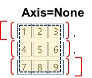
NumPy의 모든 집계 함수는 집계 함수는 AXIS를 기준으로 계산됩니다. 집계함수에 AXIS를 지정하지 않으면 axis=None입니다. axis=None, 0, 1은 다음과 같은 기준으로 생각할 수 있습니다.
- axis=None
- aixs=None은 전체 행렬을 하나의 배열로 간주하고 집계 함수의 범위를 전체 행렬로 정의합니다.
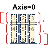
- axis=0
- aixs=0은 행을 기준으로 각 행의 동일 인덱스의 요소를 그룹으로 합니다.
- 각 그룹을 집계 함수의 범위로 정의합니다.
- axis=1
- aixs=1은 열을 기준으로 각 열의 요소를 그룹으로 합니다.
- 각 그룹을 집계 함수의 범위로 정의합니다.
- axis 관련해서는 Numpy에서 np.sum 함수의 axis 이해를 참조하시기 바랍니다.
# arange로 1부터 10미만의 범위에서 1씩 증가하는 배열 생성
# 배열의 shape을 (3, 3)으로 지정
a = np.arange(1, 10).reshape(3, 3)
pprint(a)
[ndarray 배열 객체].sum(), np.sum(): 합계
지정된 axis를 기준으로 요소의 합을 반환합니다.
a.sum(), np.sum(a)
a.sum(axis=0), np.sum(a, axis=0)
a.sum(axis=1), np.sum(a, axis=1)
[ndarray 배열 객체].min(), np.min(): 최소값
지정된 axis를 기준으로 요소의 최소값을 반환합니다.
a.min(), np.min(a)
a.min(axis=0), np.min(a, axis=0)
a.min(axis=1), np.min(a, axis=1)
[ndarray 배열 객체].max(), np.max(): 최대값
지정된 axis를 기준으로 요소의 최대값을 반환합니다.
a.max(), np.max(a)
a.max(axis=0), np.max(a, axis=0)
a.max(axis=1), np.max(a, axis=1)
[ndarray 배열 객체].cumssum(), np.cumsum(): 누적 합계
지정된 axis를 기준으로 각 요소의 누적 합의 결과를 반환합니다.
a.cumsum(), np.cumsum(a)
a.cumsum(axis=0), np.cumsum(a, axis=0)
a.cumsum(axis=1), np.cumsum(a, axis=1)
[ndarray 배열 객체].mean(), np.mean(): 평균
지정된 axis를 기준으로 요소의 평균을 반환합니다.
a.mean(), np.mean(a)
a.mean(axis=0), np.mean(a, axis=0)
a.mean(axis=1), np.mean(a, axis=1)
np.mean(): 중앙값
지정된 axis를 기준으로 요소의 중앙값을 반환합니다.
np.median(a)
np.mean(a, axis=0)
np.mean(a, axis=1)
np.corrcoef(): (상관계수)Correlation coeficient
np.corrcoef(a)
[ndarray 배열 객체].std(), np.std(): 표준편차
지정된 axis를 기준으로 요소의 표준 편차를 계산합니다.
a.std(), np.std(a)
a.std(axis=0), np.std(a, axis=0)
a.std(axis=1), np.std(a, axis=1)
7.2 브로드캐스팅
Shape이 같은 두 배열에 대한 이항 연산은 배열의 요소별로 수행됩니다. 두 배열 간의 Shape이 다를 경우 두 배열 간의 형상을 맞추는 <그림 2>의 Broadcasting 과정을 거칩니다.
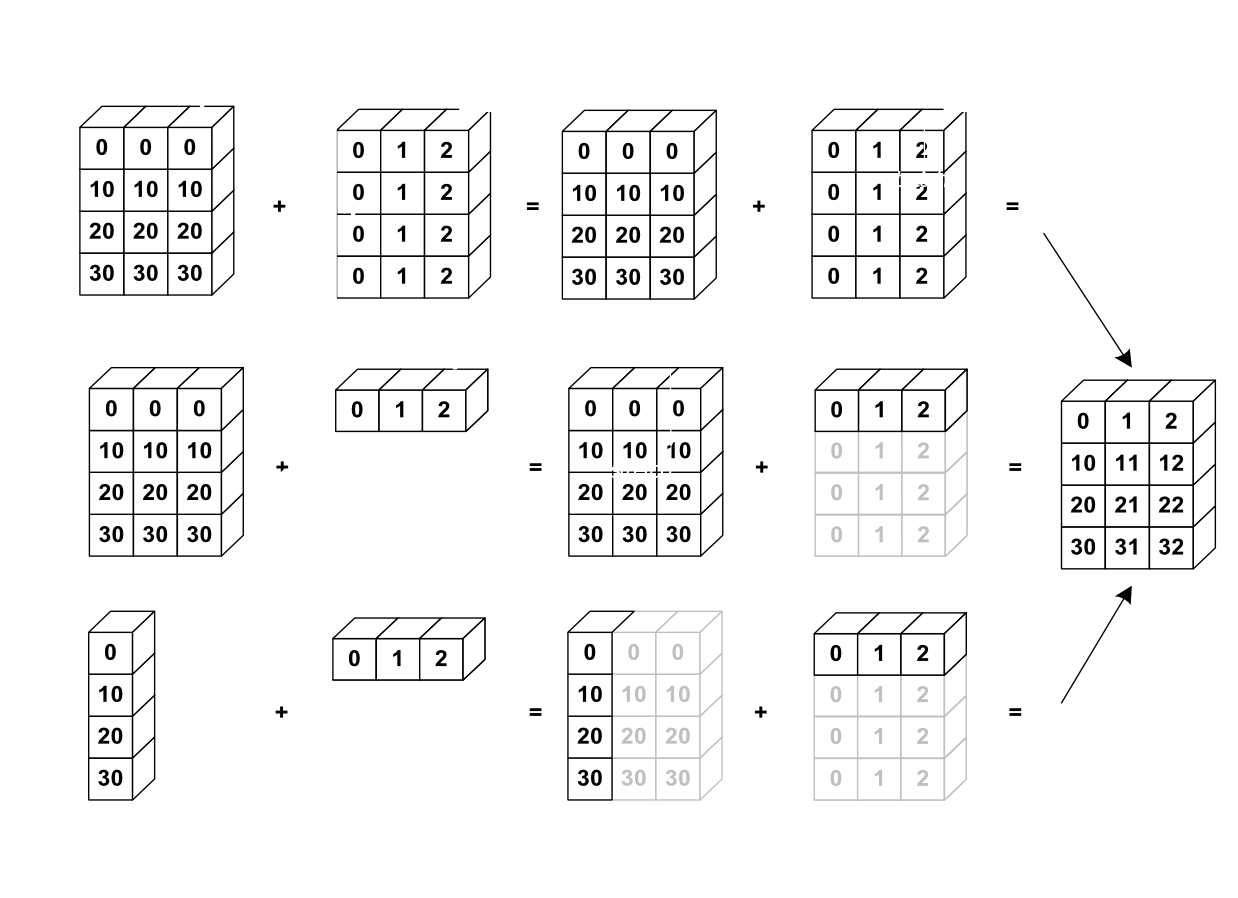
그림 2: 브로드캐스트 작동 원리
# 데모 배열 생성
a = np.arange(1, 25).reshape(4, 6)
pprint(a)
b = np.arange(25, 49).reshape(4, 6)
pprint(b)
Shape이 같은 배열의 이항 연산
- Shape이 같은 두 배열을 이항 연살 할 경우 위치가 같은 요소 단위로 수행됩니다.
a+b
Shape이 다른 두 배열의 연산
- Shape이 다른 두 배열 사이의 이항 연산에서 브로드케스팅 발생
- 두 배열을 같은 Shape으로 만든 후 연산을 수행
Case 1: 배열과 스칼라
배열과 스칼라 사이의 이항 연산 시 스칼라를 배열로 변형합니다.
# 데모 배열 생성
a = np.arange(1, 25).reshape(4, 6)
pprint(a)
a+100
- a + 100은 다음과 같은 과정을 거쳐 처리 됩니다.
# step 1: 스칼라 배열 변경
new_arr = np.full_like(a, 100)
pprint(new_arr)
# step 2: 배열 이항 연산
a+new_arr
Case 2: Shaep이 다른 배열들의 연산
# 데모 배열 생성
a = np.arange(5).reshape((1, 5))
pprint(a)
b = np.arange(5).reshape((5, 1))
pprint(b)
a+b
7.3 백터연산
NumPy는 벡터 연산을 지원합니다. NumPy의 집합 연산에는 Vectorization이 적용되어 있습니다. 배열 처리에 대한 벡터 연산을 적용할 경우 처리 속도가 100배 이상 향상됩니다. 머신러닝에서 선형대수 연산을 처리할 때 매우 높은 효과가 있을 수 있습니다.
아래 테스트에서 천만 개의 요소를 갖는 배열의 요소를 합산하는 코드를 반복문으로 처리하면 2.5초가 소요됩니다. 이 연산을 벡터 연산으로 처리하면 10밀리세컨드로 단축됩니다.
import numpy as np
# sample array
a = np.arange(10000000)
- loop 문을 이용한 연산: 처리 2.7초
result = 0
%%time
for v in a:
  result += v
result
- numpy의 벡터연산: 10 ms
%%time
result = np.sum(a)
result
8. 배열 복사
ndarray 배열 객체에 대한 slice, subset, indexing이 반환하는 배열은 새로운 객체가 아닌 기존 배열의 뷰입니다. 반환한 배열의 값을 변경하면 원본 배열에 반영됩니다. 따라서 기본 배열로부터 새로운 배열을 생성하기 위해서는 copy 함수로 명시적으로 사용해야 합니다. copy 함수로 복사된 원본 배열과 사본 배열은 완전히 다른 별도의 객체입니다.
[ndarray 배열 객체].copy(), np.copy()
#데모용 배열
a = np.random.randint(0, 9, (3, 3))
pprint(a)
copied_a1 =np.copy(a)
# 복사된 배열의 요소 업데이트
copied_a1[:, 0]=0 #배열의 전체 row의 첫번째 요소 0으로 업데이트
pprint(copied_a1)
# 복사본 배열 변경이 원보에 영향을 미치지 않음
pprint(a)
#np.copy()를 이용한 복사
copied_a2 = np.copy(a)
pprint(copied_a2)
9. 배열 정렬
ndarray 객체는 axis를 기준으로 요소 정렬하는 sort 함수를 제공합니다.
#배열 생성
unsorted_arr = np.random.random((3, 3))
pprint(unsorted_arr)
#데모를 위한 배열 복사
unsorted_arr1 = unsorted_arr.copy()
unsorted_arr2 = unsorted_arr.copy()
unsorted_arr3 = unsorted_arr.copy()
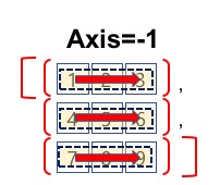
- [ndarray 객체].sort() axis의 기본 값은 -1입니다.
- axis=-1은 현재 배열의 마지막 axis를 의미합니다.
- 현재 unsorted_arr의 마지막 axis는 1입니다.
- [ndarray 객체].sort()와 [ndarray 객체].sort(axis=1)의 결과는 동일합니다.
#배열 정렬
unsorted_arr1.sort()
pprint(unsorted_arr1)
- axis=0의 정렬 방향은 다음 그림과 같습니다.
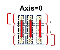
#배열 정렬, axis=0
unsorted_arr2.sort(axis=0)
pprint(unsorted_arr2)
- axis=1의 정렬 방향은 다음 그림과 같습니다.
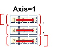
#배열 정렬, axis=1
unsorted_arr3.sort(axis=1)
pprint(unsorted_arr3)
10. 서브셋, 슬라이싱, 인덱싱
배열의 개별 요소, 요소 집합을 참조하는 방법을 소개합니다.
10.1 요소 선택
배열의 각 요소는 axis 인덱스 배열로 참조할 수 있습니다. 1차원 배열은 1개 인덱스, 2차원 배열은 2개 인덱스, 3차원 인덱스는 3개 인덱스로 요소를 참조할 수 있습니다.
인덱스로 참조한 요소는 값 참조, 값 수정이 모두 가능합니다.
# 데모 배열 생성
a0 = np.arange(24) # 1차원 배열
pprint(a0)
a1 = np.arange(24).reshape((4, 6)) #2차원 배열
pprint(a1)
a2 = np.arange(24).reshape((2, 4, 3)) # 3차원 배열
pprint(a2)
1 차원 배열 요소 참조 및 변경
a0[5] # 5번 인덱스 요소 참조
# 5번 인덱스 요소 업데이트
a0[5] = 1000000
pprint(a0)
2 차원 배열 요소 참조 및 변경
pprint(a1)
# 1행 두번째 컬럼 요소 참조
a1[0, 1]
# 1행 두번째 컬럼 요소 업데이트
a1[0, 1]=10000
pprint(a1)
3 차원 배열 요소 참조 및 변경
pprint(a2)
# 2 번째 행, 첫번째 컬럼, 두번째 요소 참조
a2[1, 0, 1]
a2[1, 0, 1]=10000
pprint(a2)
10.2 슬라이싱(Slicing)
여러개의 배열 요소를 참조할 때 슬라이싱을 사용합니다. 슬라이싱은 axis 별로 범위를 지정하여 실행합니다. 범위는 $from_index:to_index$ 형태로 지정합니다. from_index는 범위의 시작 인덱스이며, to_index는 범위의 종료 인덱스입니다. 요소 범위를 지정할 때 to_index는 결과에 포함되지 않습니다. $from_index:to_index$의 범위 지정에서 from_index는 생략 가능합니다. 생략할 경우 0을 지정한 것으로 간주합니다. to_index 역시 생략 가능합니다. 이 경우 마지막 인덱스로 설정됩니다. 따라서 “$:$” 형태로 지정된 범위는 전체 범위를 의미합니다.
from_index와 to_index에 음수를 지정하면 이것은 반대 방향을 의미합니다. 예를 들어서 -1은 마지막 인덱스를 의미합니다.
슬라이싱은 원본 배열의 뷰입니다. 따라서 슬라이싱 결과의 요소를 업데이트하면 원본에 반영됩니다.
# 데모 배열 생성
a1 = np.arange(1, 25).reshape((4, 6)) #2차원 배열
pprint(a1)
가운데 요소 가져오기
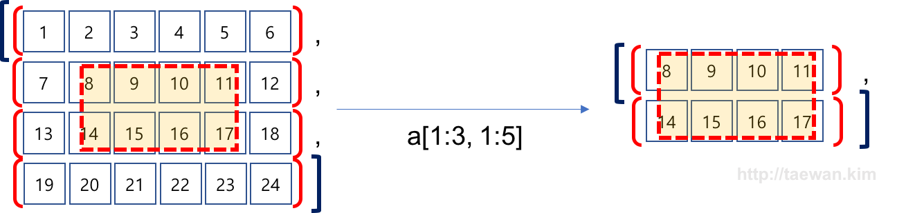
a1[1:3, 1:5]
- 음수 인덱스를 이용한 범위 설정
- 음수 인덱스는 지정한 axis의 마지막 요소로 부터 반대 방향의 인덱스입니다.
- -1은 마지막 요소의 인덱스를 의미합니다.
- 다음 슬라이싱은 위 슬라이싱과 동일한 결과를 만듭니다.
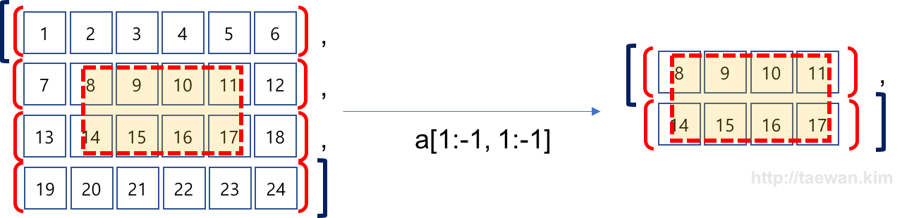
a1[1:-1, 1:-1]
슬라이싱 업데이트
# 데모 대상 배열 조회
pprint(a1)
# 슬라이싱 배열
slide_arr = a1[1:3, 1:5]
pprint(slide_arr)
# 슬라이싱 결과 배열에 슬라이싱을 적용하여 4개 요소 참조
slide_arr[:, 1:3]
pprint(slide_arr)
# 슬라이싱을 적용하여 참조한 4개 요소 업데이트 및 슬라이싱 배열 조회
slide_arr[:, 1:3]=99999
pprint(slide_arr)
# 원본 배열에 반영된 결과 확인
pprint(a1)
10.3 블린 인덱싱(Boolean Indexing)
NumPy는 불린 인덱싱은 배열 각 요소의 선택 여부를 True, False 지정하는 방식입니다. 해당 인덱스의 True만을 조회합니다.
# 데모 배열 생성
a1 = np.arange(1, 25).reshape((4, 6)) #2차원 배열
pprint(a1)
- a1 배열에서 요소의 값이 짝수인 요소들의 총 합은?
# 짝수인 요소 확인
# numpy broadcasting을 이용하여 짝수인 배열 요소 확인
even_arr = a1%2==0
pprint(even_arr)
# a1[a1%2==0] 동일한 의미입니다.
a1[even_arr]
np.sum(a1)
Boolean Indexing의 응용
- 2014년 시애클 강수량 데이터: ./data/seattle2014.csv
- 2014년 시애틀 1월 평균 강수량은?
!head -n 3 ./data/seattle2014.csv
# 데이터 로딩
import pandas as pd
rains_in_seattle = pd.read_csv("./data/seattle2014.csv")
rains_arr = rains_in_seattle['PRCP'].values
print("Data Size:", len(rains_arr))
# 날짜 배열
days_arr = np.arange(0, 365)
# 1월의 날수 boolean index 생성
condition_jan = days_arr < 31
# 40일 조회
condition_jan[:40]
#1월의 강수량 추출
rains_jan = rains_arr[condition_jan]
#강수량 데이터 수 (1월: 31일)
len(rains_jan)
# 1월 강수량 총합
np.sum(rains_jan)
# 1월 평균 강수향
np.mean(rains_jan)
10.4 팬시 인덱싱(Fancy Indexing)
배열에 인덱스 배열을 전달하여 요소를 참조하는 방법입니다.
11. 배열 변환
배열을 변환하는 방접으로는 전치, 배열 shape 변환, 배열 요소 추가, 배열 결합, 분리 등이 있습니다. 각 배열 변경 방법에 대하여 살펴보겠습니다.
11.1 전치(Transpose)
Tranpose는 행렬의 인덱스가 바뀌는 변환입니다. 행렬의 Tranpose의 예는 다음과 같습니다.
$$
\begin{align}
\begin{bmatrix}1&2\end{bmatrix}^T & = \begin{bmatrix}1\\2\end{bmatrix} \\
\begin{bmatrix}1&2\\3&4\end{bmatrix}^T & = \begin{bmatrix}1&3\\2&4\end{bmatrix} \\
\begin{bmatrix}1&2\\3&4\\5&6\end{bmatrix}^T & = \begin{bmatrix}1&3&5\\2&4&6\end{bmatrix}
\end{align}
$$
- 다음은 NumPy에서 행렬을 전치하기 위하여 [numpy.ndarray 객체].T 속성을 사용합니다.
- 이 속성은 전치된 행렬을 반환합니다.
# 행렬 생성
a = np.random.randint(1, 10, (2, 3))
pprint(a)
#행렬의 전치
pprint(a.T)
11.2 배열 형태 변경
[numpy.ndarray 객체]는 배열의 Shape을 변경하는 ravel 메서드와 reshape 메서드를 제공합니다.
- ravel은 배열의 shape을 1차원 배열로 만드는 메서드입니다.
- reshape은 데이터 변경없이 지정된 shape으로 변환하는 메서드입니다.
[numpy.ndarray 객체].ravel()
배열을 1차원 배열로 반환하는 메서드입니다. numpy.ndarray 배열 객체의 View를 반환합니다. ravel 메서드가 반환하는 배열은 원본 배열이 뷰입니다. 따라서 ravel 메서드가 반환하는 배열의 요소를 수정하면 원본 배열 요소에도 반영됩니다.
# 데모 배열 생성
a = np.random.randint(1, 10, (2, 3))
pprint(a)
a.ravel()
- revel이 반환하는 배열은 a 행렬의 view입니다.
- 반환 행렬의 데이터를 변경하면 a 행렬도 변경됩니다.
b = a.ravel()
pprint(b)
b[0]=99
pprint(b)
# b 배열 변경이 a 행렬에 반영되어 있습니다.
pprint(a)
[numpy.ndarray 객체].reshape()
[numpy.ndarray 객체]의 shape을 변경합니다. 실제 데이터를 변경하는 것은 아닙니다. 배열 객체의 shape 정보만을 수정합니다.
# 대상 행렬 속성 확인
a = np.random.randint(1, 10, (2, 3))
pprint(a)
result = a.reshape((3, 2, 1))
pprint(result)
11.3 배열 요소 추가 삭제
배열의 요소를 변경, 추가, 삽입 및 삭제하는 resize, append, insert, delete 함수를 제공합니다.
resize()
- np.resize(a, new_shape)
- np.ndarray.resize(new_shape, refcheck=True)
- 배열의 shape과 크기를 변경합니다.
np.resize와 np.reshape 함수는 배열의 shape을 변경한다는 부분에서 유사합니다. 차이점은 reshape 함수는 배열 요소 수를 변경하지 않습니다. reshape 전후 배열의 요소 수는 같습니다. 반면에 resize는 shape을 변경하는 과정에서 배열 요소 수를 줄이거나 늘립니다.
- 일반적인 resize 사용 방법
#배열 생성
a = np.random.randint(1, 10, (2, 6))
pprint(a)
# shape 변경 - 요소 수 변경 없음
a.resize((6, 2))
pprint(a)
- 요소 수가 늘어난 변경
#배열 생성
a = np.random.randint(1, 10, (2, 6))
pprint(a)
# 요소숙 12개에서 20개로 늘어남
# 늘어난 요소는 0으로 채워짐
a.resize((2, 10))
pprint(a)
- 요소 수가 즐어든 변경
#배열 생성
a = np.random.randint(1, 10, (2, 6))
pprint(a)
# 요소숙 12개에서 9개로 줄임
# 이전 데이터 삭제
a.resize((3, 3))
pprint(a)
append()
- np.append(arr, values, axis=None)
- 배열의 끝에 값을 추가
np.append 함수는 arr의 끝에 values(배열)을 추가합니다. axis로 배열이 추가되는 방향을 지정할 수 있습니다.
# 데모 배열 생성
a = np.arange(1, 10).reshape(3, 3)
pprint(a)
b = np.arange(10, 19).reshape(3, 3)
pprint(b)
case 1: axis을 지정하지 않을 경우
axis를 지정하지 않으면 배열은 1차원 배열로 변형되어 결합됩니다.
# axis 지정 없이 추가
result = np.append(a, b)
pprint(result)
#원본 배열을 변경하는 것이 아니며 새로운 배열이 생성됩니다.
pprint(a)
case 2: axis=0 지정
# axis = 0
# axis 0 방향으로 b 배열 추가
result = np.append(a, b, axis=0)
pprint(result)
- axis = 0 설정 시, shape[0]를 제외한 나머지 shape은 같아야 합니다.
- shape[0]를 제외한 나머지 shape이 다를 경우 append는 오류를 발생합니다.
different_sahpe_arr = np.arange(10, 20).reshape(2, 5)
pprint(different_sahpe_arr)
# 기준 축을 제외한 shape이 다른 배열의 append: 오류 발생
np.append(a, different_sahpe_arr, axis=0)
case 3: axis=1 지정
- axis = 1 설정 시, shape[1]을 제외한 나머지 shape은 같아야 합니다.
- shape[1]를 제외한 나머지 shape이 다를 경우 append는 오류를 발생합니다.
# axis = 1
# axis 1 방향으로 b 배열 추가
result = np.append(a, b, axis=1)
pprint(result)
- axis = 1 설정 시, shape[1]를 제외한 나머지 shape은 같아야 합니다.
- shape[1]를 제외한 나머지 shape이 다를 경우 append는 오류를 발생합니다.
# shape이 다른 배열 생성
different_sahpe_arr = np.arange(10, 20).reshape(5, 2)
pprint(different_sahpe_arr)
# 기준 축을 제외한 shape이 다른 배열의 append: 오류 발생
np.append(a, different_sahpe_arr, axis=1)
insert()
- np.insert(arr, obj, values, axis=None)
- axis를 지정하지 않으며 1차원 배열로 변환
- 추가할 방향을 axis로 지정
# 데모 배열 생성
a = np.arange(1, 10).reshape(3, 3)
pprint(a)
# a 배열을 일차원 배열로 변환하고 1번 index에 99 추가
np.insert(a, 1, 999)
# a 배열의 axis 0 방향 1번 인덱스에 추가
# index가 1인 row에 999가 추가됨
np.insert(a, 1, 999, axis=0)
# a 배열의 axis 1 방향 1번 인덱스에 추가
# index가 1인 column에 999가 추가됨
np.insert(a, 1, 999, axis=1)
delete()
- np.delete(arr, obj, axis=None)
- axis를 지정하지 않으며 1차원 배열로 변환
- 삭제할 방향을 axis로 지정
- delete 함수는 원본 배열을 변경하지 않으며 새로운 배열을 반환
# 데모 배열 생성
a = np.arange(1, 10).reshape(3, 3)
pprint(a)
# a 배열을 일차원 배열로 변환하고 1번 index 삭제
np.delete(a, 1)
# a 배열의 axis 0 방향 1번 인덱스인 행을 삭제한 배열을 생성하여 반환
np.delete(a, 1, axis=0)
# a 배열의 axis 1 방향 1번 인덱스인 열을 삭제한 배열을 생성하여 반환
np.delete(a, 1, axis=1)
11.4 배열 결합
배열과 배열을 결합하는 np.concatenate, np.vstack, np.hstack 함수를 제공합니다.
배열 결합
np.concatenate
- concatenate((a1, a2, ...), axis=0)
- a1, a2....: 배열
# 데모 배열
a = np.arange(1, 7).reshape((2, 3))
pprint(a)
b = np.arange(7, 13).reshape((2, 3))
pprint(b)
# axis=0 방향으로 두 배열 결합, axis 기본값=0
result = np.concatenate((a, b))
result
# axis=0 방향으로 두 배열 결합, 결과 동일
result = np.concatenate((a, b), axis=0)
result
# axis=1 방향으로 두 배열 결합, 결과 동일
result = np.concatenate((a, b), axis=1)
result
수직 방향 배열 결합
np.vstack
- np.vstack(tup)
- tup: 튜플
- 튜플로 설정된 여러 배열을 수직 방향으로 연결 (axis=0 방향)
- np.concatenate(tup, axis=0)와 동일
# 데모 배열
a = np.arange(1, 7).reshape((2, 3))
pprint(a)
b = np.arange(7, 13).reshape((2, 3))
pprint(b)
np.vstack((a, b))
# 4개 배열을 튜플로 설정
np.vstack((a, b, a, b))
수평 방향 배열 결합
np.hstack
- np.hstack(tup)
- tup: 튜플
- 튜플로 설정된 여러 배열을 수평 방향으로 연결 (axis=1 방향)
- np.concatenate(tup, axis=1)와 동일
# 데모 배열
a = np.arange(1, 7).reshape((2, 3))
pprint(a)
b = np.arange(7, 13).reshape((2, 3))
pprint(b)
np.hstack((a, b))
np.hstack((a, b, a, b))
11.5 배열 분리
NumPy는 배열을 수직, 수평으로 분할하는 함수를 제공합니다.
- np.hsplit(): 지정한 배열을 수평(행) 방향으로 분할
- np.vsplit(): 지정한 배열을 수직(열) 방향으로 분할
배열 수평 분할
- np.hsplit(ary, indices_or_sections)
- 배열을 수평 방향(컬럼 방향)으로 분할하는 함수
# 분할 대상 배열 생성
a = np.arange(1, 25).reshape((4, 6))
pprint(a)
수평 방향으로 배열을 두 그룹으로 분할
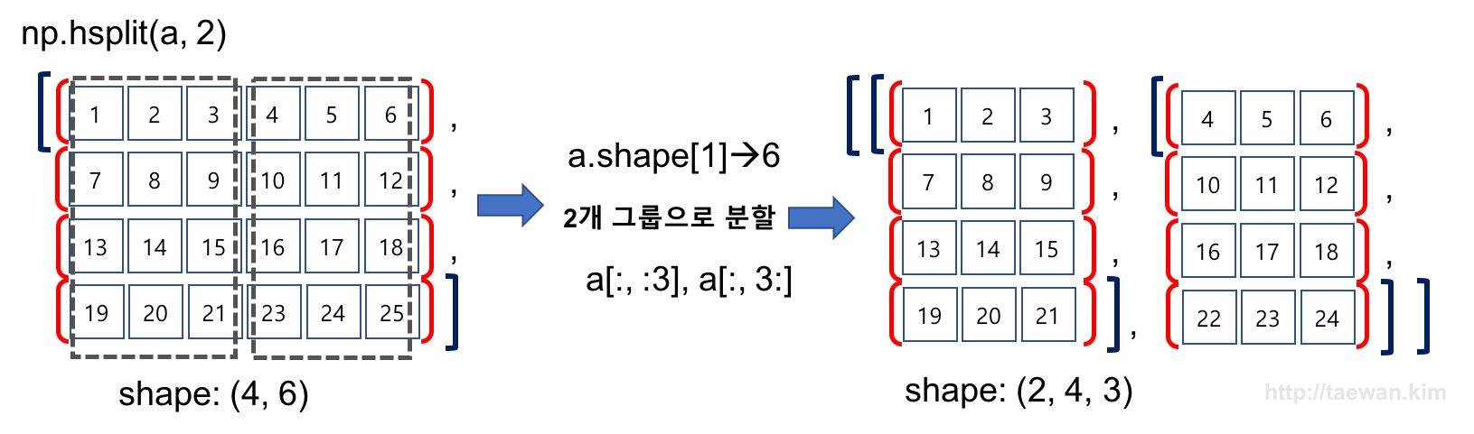
# 수평으로 두 그룹으로 분할하는 함수
result = np.hsplit(a, 2)
result
수평 방향으로 배열을 세 그룹으로 분할
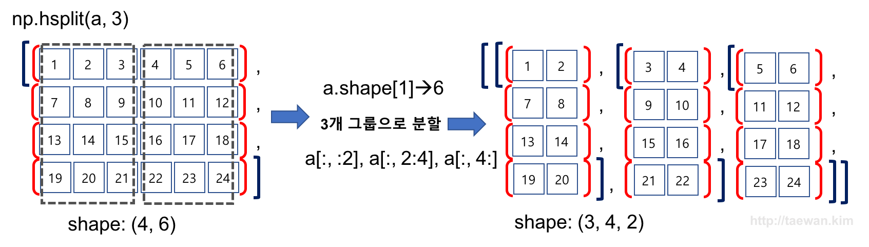
# 수평으로 두 그룹으로 분할하는 함수
result = np.hsplit(a, 3)
result
수평 방향으로 여러 구간으로 구분
- np.hsplit의 두 번째 파라미터에 구간 설정 배열을 전달하여 여러 배열로 구분합니다.
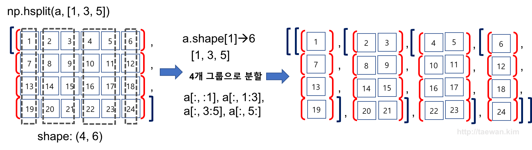
np.hsplit(a, [1, 3 ,5])
배열 수직 분할
- np.vsplit(ary, indices_or_sections)
- 배열을 수직 방향(행 방향)으로 분할하는 함수
# 분할 대상 배열 생성
a = np.arange(1, 25).reshape((4, 6))
pprint(a)
수직 방향으로 배열을 두 개 그룹으로 분할
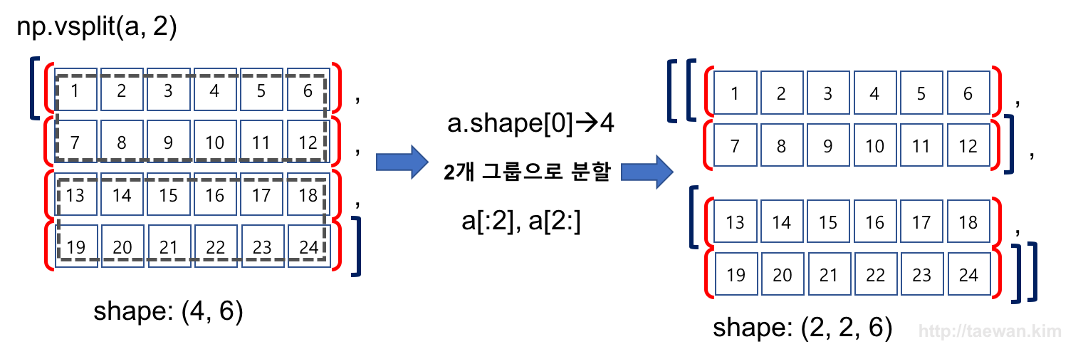
result=np.vsplit(a, 2)
result
np.array(result).shape
수직 방향으로 배열을 4 개 그룹으로 분할
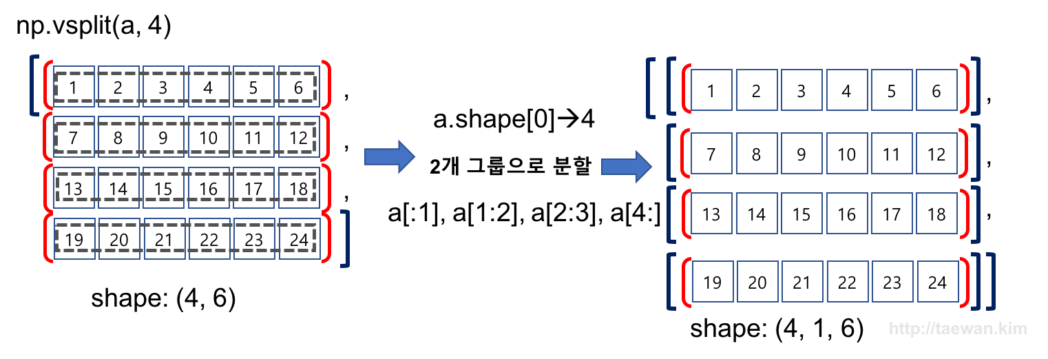
result=np.vsplit(a, 4)
result
np.array(result).shape
수직 방향으로 여러 구간으로 구분
- np.hsplit의 두 번째 파라미터에 구간 설정 배열을 전달하여 여러 배열로 구분합니다.
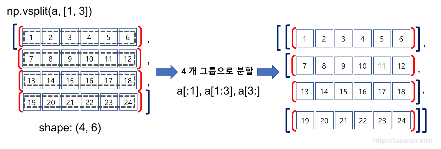
# row를 1, 2-3, 4번째 라인으로 구분
np.vsplit(a, [1, 3])
12. 참고자료
- Python Numpy Tutorial - http://cs231n.github.io/
- Python For Data Science Cheat Sheet NumPy Basics by DataCamp
- docs.scipy.org: Quickstart tutorial
- Numpy는 /NUM-pee/ 혹은 /NUM-pai/ 로 발음합니다. https://www.youtube.com/watch?v=Uqd7pgpO2-g [return]